What makes gold a strategic asset?

Gold has a key role as a strategic long-term investment and as a mainstay allocation in a well-diversified portfolio. Investors have been able to recognise much of gold’s value over time by maintaining a long-term allocation and taking advantage of its safe-haven status during periods of economic uncertainty.

Gold is a highly liquid asset, which is no one’s liability, carries no credit risk, and is scarce, historically preserving its value over time. It also benefits from diverse sources of demand: as an investment, a reserve asset, gold jewellery, and a technology component. These attributes mean gold can enhance a portfolio in three key ways:

• Delivering long-term returns

• Improving diversification

• Providing liquidity

Combined, these characteristics make gold a clear complement to stocks and bonds and a welcome addition to broad-based portfolios.

Moreover, the shift towards a greater integration of environmental, social and governance (ESG) objectives within investment strategies has important implications and we believe gold can play a role in supporting these. Gold – from established investment sources – should be recognised as an asset that is responsibly produced and delivered from a supply chain that adheres to high ESG standards. Gold also has a potential role to play in reducing investor exposure to climate-related risks.

Gold's key attributes

A long-term source of return

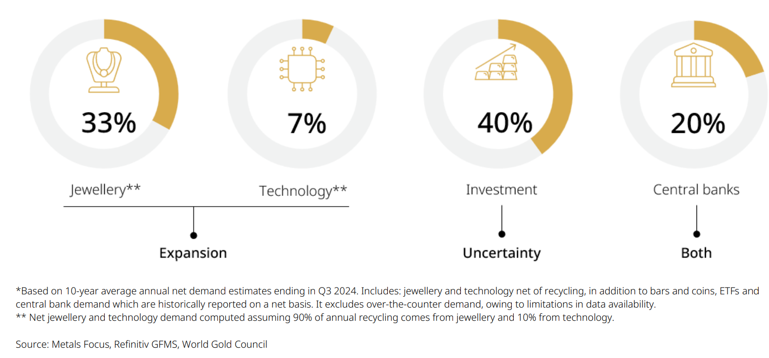
Investors have long considered gold a beneficial asset during periods of uncertainty. Yet, historically, it has generated long-term positive returns in both good and bad economic times. Its diverse sources of demand give gold a particular resilience and the potential to deliver solid returns in various market conditions (Figure 1). Gold is, on the one hand, often used as an investment to protect and enhance wealth over the long term, but on the other hand it is also a consumer good, via jewellery and technology demand. During periods of economic uncertainty, it is the counter-cyclical investment demand that drives the gold price up. During periods of economic expansion, the pro-cyclical consumer demand supports its performance.

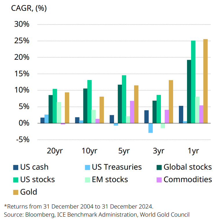
Looking back over more-than half a century since the US gold standard collapsed in 1971, the price of gold in US dollars has increased by 8% on an annualised basis – a performance comparable with that of equities and higher than that of bonds over the same period. Gold has also outperformed many other major asset classes over the past 1, 3, 5, 10 and 20 years (Chart 1).

The fact that gold has performed so well is no coincidence. Our research shows that the gold price over the long term is primarily driven by an economic component balanced by a financial component. We call this approach Gold’s Long Term Expected return (GLTER).

Figure 1: Gold’s sources of demand Average annual net demand = 3,034 tonnes* (approx. US$233bn)

GLTER’s robust framework builds upon the composition and drivers of above-ground gold stocks. The model suggests that gold’s long-run return closely mirrors global GDP and is, therefore, materially higher than inflation. This also implies that gold should be viewed as an asset that can positively contribute to long-term portfolio returns, supplementing its wellestablished role as a hedge.

Chart 1: Gold has performed well over the past 1, 3, 5, 10 and 20 years, despite the strong performance of risk assets

Annualised return over the past 1, 3, 5, 10 and 20 years*

Gold in US dollars has increased by 8% per year since 1971

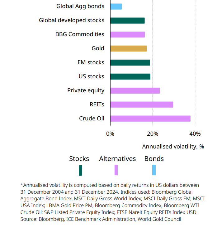
Moreover, the diversity of its sources of demand help to make gold a less volatile asset than some equity indices, other commodities or alternatives (Chart 2).

Chart 2: Gold has been less volatile than many equity indices, alternatives and commodities because of its scale, liquidity and diverse sources of demand

Average daily volatility of several major assets since 2004*

Beating inflation, combating deflation

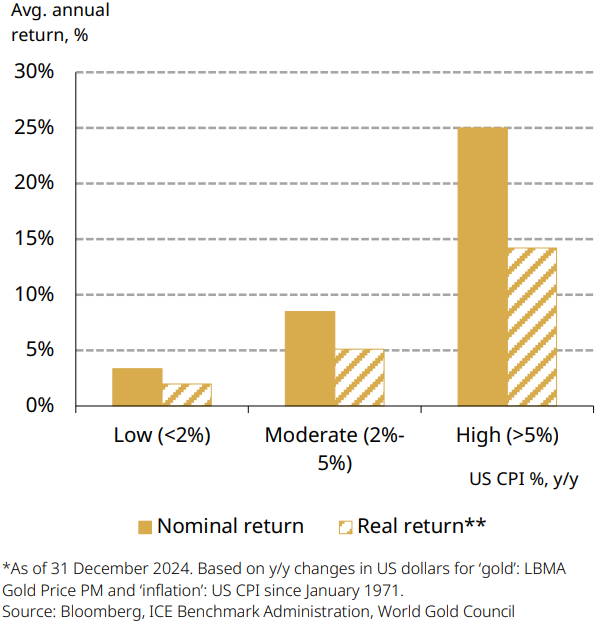
Gold has long been considered a hedge against inflation and the data confirms this: since 1971 it has outpaced the US and world consumer price indices (CPI).1 Gold also protects investors against high inflation. In years when inflation was between 2%- 5%, gold’s price increased 8% per year on average. This number increased significantly with even higher inflation levels (Chart 3). Over the long term, therefore, gold has not just preserved capital but also helped it grow.

Chart 3: Gold historically rallies in periods of high inflation

Gold nominal and real returns in US dollars as a function of annual inflation*

Our research also shows that gold should do well in periods of deflation. Such periods are characterised by low interest rates, reduced consumption and investment, and financial stress, all of which tend to foster gold demand.

Store of value

Historically, major currencies were pegged to gold. That changed with the unravelling of the US gold standard in 1971 and the eventual collapse of the Bretton Woods system. Since then, with few exceptions, gold has significantly outperformed all major currencies and commodities as a means of exchange. And although this outperformance was particularly marked immediately following the end of the gold standard, gold has clearly continued to outperform most major currencies in the more recent past (Chart 4). A key factor behind this robust performance is that gold mine production has grown slowly over time – increasing by approximately 1.7% per year over the past 20 years.

Chart 4: The purchasing power of major currencies and commodities has significantly eroded relative to gold

Value of currencies and broad commodities relative to gold (January 2000 = 100)*

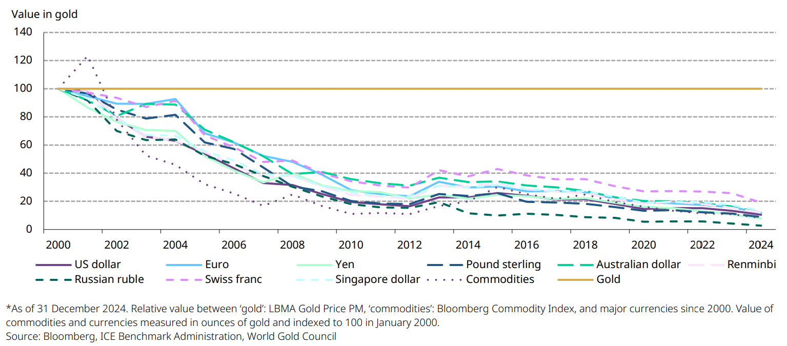
By contrast, fiat money can be printed in unlimited quantities to support monetary policy. This is clearly exemplified by the quantitative easing (QE) measures implemented in the aftermath of the Global Financial Crisis (GFC) and the COVID-19 pandemic. These crises saw many investors turn to gold to hedge themselves against currency devaluation and preserve their purchasing power over time.

The environment catalysed by QE created optimal conditions for gold to perform well, tracking the rapid expansion in the US money supply (Chart 5).2

Chart 5: Gold prices have tracked the expansion of US money supply

US M2 growth, US CPI and gold price* 

Diversification that works

Effective diversifiers are sometimes hard to find. Many assets become increasingly correlated as market uncertainty rises and volatility is more pronounced, driven in part by risk-on/risk-off investment decisions. As a result, many so-called diversifiers fail to protect portfolios when investors need them most.

Gold is different in that its negative correlation to equities and other risk assets increases as these assets sell off (Chart 6). The GFC is a case in point. Equities and other risk assets tumbled in value, as did hedge funds, real estate and most commodities, which were long deemed portfolio diversifiers. Gold, by contrast, held its own and increased in price, rising 21% in US dollars from December 2007 to February 2009. And in the most recent sharp equity market pullbacks of 2020 and 2022, gold’s performance remained positive.

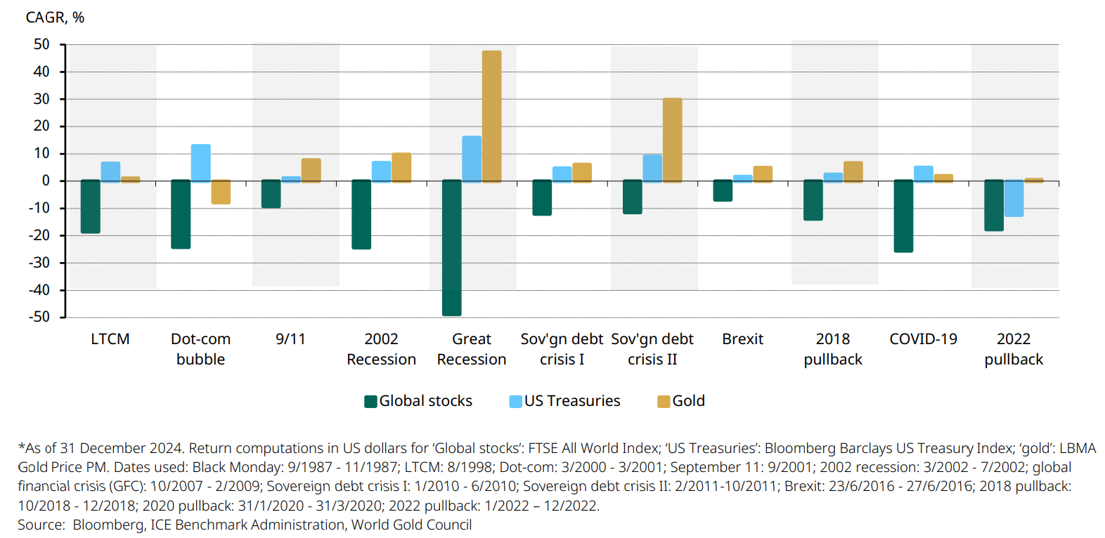
This robust performance is not surprising. With few exceptions, gold has been particularly effective during times of systemic risk, delivering positive returns and reducing overall portfolio losses (Chart 7).

Chart 6: Gold becomes more negatively correlated with stocks in extreme market selloffs

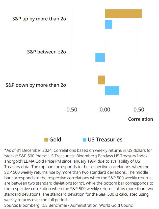
Chart 7: The gold price tends to increase in periods of systemic risk

Stocks, bonds and gold during various crises*

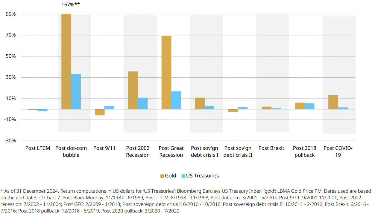
But gold’s correlation does not just work for investors during periods of turmoil. It can also deliver positive correlation with equities and other risk assets in positive markets, making gold a well-rounded efficient hedge (Chart 8).

This benefit arises from gold’s dual nature: as both an investment and a consumer good. As such, the longterm performance of gold is supported by income growth. Our analysis bears this out, showing that when equities rally strongly their correlation to gold can increase. This is driven by a wealth effect supporting gold consumer demand, as well as demand from investors seeking protection against higher inflation expectations.

Gold has a dual nature as both an investment and a consumer good

Chart 8: Gold performs well in the recovery periods following a systemic selloff

Performance of gold and Treasuries from the market trough (bottom) to the market recovery point (stock market levels before the systemic selloff)*

A deep and liquid market

The gold market is large, global, and highly liquid. We estimate that physical gold holdings by investors and central banks are worth approximately US$5.1tn, with an additional US$1.0tn in open interest through derivatives traded on exchanges or the over-thecounter (OTC) market.

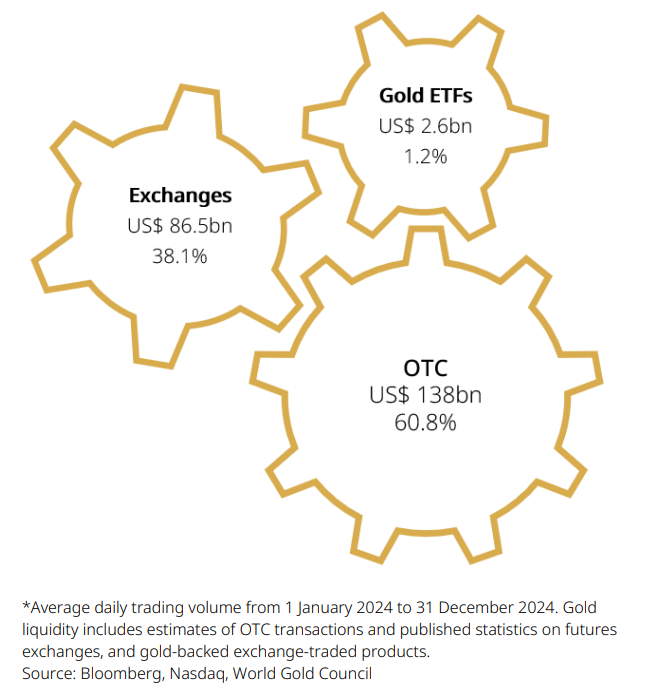
The gold market is also more liquid than several major financial markets, including euro/yen and the Dow Jones Industrial Average, while trading volumes are similar to those of US T-Bills (Chart 9). Gold’s trading volumes averaged approximately US$163bn per day in 2023. During that period, OTC spot and derivatives contracts accounted for US$99bn and gold futures traded US$62bn per day across various global exchanges. Physically-backed gold ETFs (gold ETFs) offer an added source of liquidity, with global gold ETFs trading an average of US$2bn per day (Chart 10)

Chart 9: Gold trades more than many other major financial assets

Average daily trading volumes over the last year in US dollars*

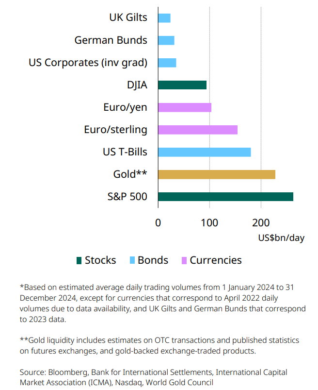
Gold's trading volumes averaged approximately US$227bn per day in 2024

Chart 10: Gold is liquid across key investment platforms

Average daily trading volume by point of access in 2024*

The scale and depth of the market means that it can comfortably accommodate large, buy-and-hold institutional investors. In stark contrast to many financial markets, gold’s liquidity does not dry up, even at times of financial stress. Importantly too, gold allows investors to meet liabilities when less liquid assets in their portfolio are difficult to sell, or are mispriced.

Portfolio impact

Risk/reward profile

Long-term returns, liquidity and effective diversification all benefit overall portfolio performance. In combination, they suggest that the addition of gold can materially enhance a portfolio’s risk-adjusted returns.

Our analysis of investment performance over the past 3, 5, 10 and 20 years emphasises gold’s positive impact on an institutional portfolio (Chart 11).

Chart 11: Hypothetical portfolio

Asset allocation: 50% stocks, 40% fixed income, 10% alternatives*

Table 1: Gold has increased risk-adjusted returns while reducing portfolio volatility and maximum drawdowns

Comparison of a hypothetical USD portfolio and an equivalent portfolio with 5% gold over the past 3, 5, 10 and 20 years based on US-dollar returns*

It shows that an average USD portfolio would have achieved higher risk-adjusted returns and lower drawdowns if 2.5%, 5%, 7.5% or 10% were allocated to gold (Chart 12 and Table 1).

Chart 12: Adding gold over the past 20 years would have increased risk-adjusted returns of a hypothetical USD portfolio

Risk-adjusted returns of a hypothetical portfolio with and without gold*

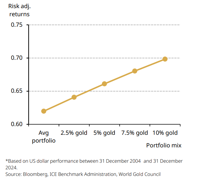
Chart 13: Gold could significantly improve risk-adjusted portfolio returns across various levels of risk

Efficient frontier of a hypothetical average portfolio*

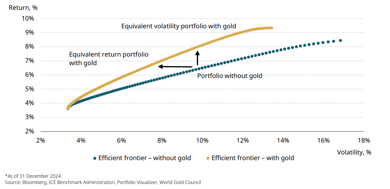
In addition to a traditional historical simulation, a mean variance optimisation analysis suggests that an allocation to gold may result in a material enhancement to portfolio risk-adjusted returns by shifting the efficient frontier upwards. For example, a portfolio with gold could deliver a higher return for the same level of risk, or the same return for a lower level of risk (Chart 13).

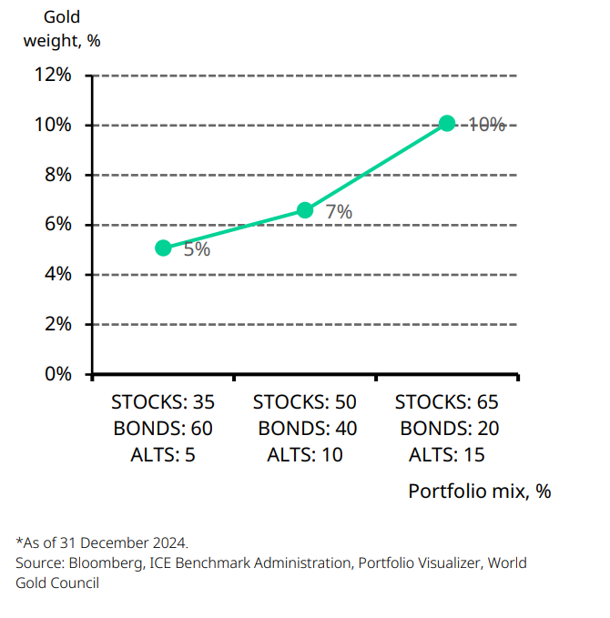
The ‘optimal’ amount of gold varies according to individual asset allocation decisions. Broadly speaking, the analysis suggests that the higher the risk in the portfolio – whether in terms of volatility or concentration of assets – the larger the required allocation to gold, within the range in consideration to offset that risk (Chart 14).

Gold may result in a material enhancement to portfolio risk-adjusted returns

Chart 14: The optimal gold allocation varies depending on the level of risk in the portfolio

The gold allocation that could deliver the maximum risk-adjusted return for each hypothetical portfolio mix

Gold’s ESG credentials and contributions

While gold mining is, by definition, an extractive industry, responsible gold miners follow stringent frameworks to mitigate environmental impact and reduce risks. In fact, the social and economic contribution of the gold mining industry plays a key role in the communities and host countries in which it operates. It does so through the payment of wages and taxes, supporting local economic development, improving infrastructure, providing access to healthcare and schooling, and much more. The majority of this expenditure remains in the local economies of host nations and communities, as documented recently in our measurement of the social and economic contribution of gold mining. The industry is also committed to contributing to the advancement of the UN Sustainable Development Goals.

In addition, gold has a potential role to play in reducing investor exposure to climate-related risks. In fact, gold’s lack of downstream emissions has important implications, as gold holdings can reduce the overall carbon intensity of the portfolio value. And the positive outlook for future decarbonisation of the gold value chain has potential benefits for the projected carbon profile, ‘implied temperature’ and climate target alignment of portfolio holdings.

Our analysis suggests that gold has the potential to perform better than many mainstream asset classes under various long-term climate scenarios, particularly if climate impacts create or exacerbate market volatility or we experience a disruptive transition to a net zero carbon economy. Furthermore, gold’s value is less likely to be negatively impacted by a rising carbon price, also offering investors a degree of insulation from the likely policy responses needed to accelerate the move to a decarbonised economy.

Gold also has a potential role to play in reducing exposure to climate-related risks

Potential risks and challenges

Given the risk/reward trade off associated with any investment, it is important to acknowledge and understand not only opportunities, but also key risks.

No cash flows: A widely perceived drawback of gold is that it does not provide a regular income, unlike other asset classes such as bonds, property or even some company stocks. But the reason for this is simple: gold has no credit risk. There is no promise to repay. Nor does it bear any counter-party risk. This means, however, that investors depend on price appreciation to benefit from gold. And in this regard gold has a good track record. It has generated long-term positive returns in both good and bad economic times. At the same time, gold has outperformed many other major asset classes over various investment horizons (3, 5, 10, 20 and 50 years).3

Gold’s strong performance is no coincidence: it is a byproduct of its underlying demand and supply dynamics, which combine a natural scarcity with diverse sources of demand including jewellery, technology, investment and central banks.

Price volatility: Gold is a great diversifier to a portfolio because it behaves so differently to equities and bonds, not because it has a low volatility. And while gold is a less volatile asset than some equity indices, other commodities or alternatives, in some years the metal has posted close to 30% gains (2010) and in other years it has posted close to 30% losses (2013). On balance, however, gold has an asymmetric correlation profile with equities; in other words, it does much better when equities fall than it does badly when equities rise.

Conclusion

Perceptions of gold have changed substantially over the past two decades, reflecting increased wealth in the East and a growing worldwide appreciation of gold’s role within an institutional investment portfolio.

Gold’s unique attributes as a scarce, highly liquid and uncorrelated asset enable it to act as a diversifier over the long term. Gold’s position as an investment and a luxury good has allowed it to deliver annualised returns of 8% since 1971, comparable to equities and more than bonds and commodities.

Gold’s traditional role as a safe-haven asset means it comes into its own during times of high risk. But its dual appeal as an investment and a consumer good means it can generate positive returns in good times too. This dynamic is likely to continue, reflecting ongoing political and economic uncertainty, and economic concerns surrounding equity and bond markets.